
Tip
See our video guides for quick tutorials that walk you through Sigmacalx basic functionalities and concepts. This is the easiest and quickest way to get going with Sigmacalx forms.
Von Mises stress is an equivalent stress value based on distortion energy that shows if a material will yield or fracture under a given loading condition. It is mostly used for ductile materials, such as metals.
Material failure envelope is represented as an ellipse or a circle drawn in all four quadrants on cartesian system. Each quadrant represents a pair of loads (pressure and axial load). Positive axes on the cartesian system represent either internal pressure or tensile load. Negative axes on the cartesian system represent either external pressure or compressive load.
Below is a common example of failure envelope of a ductile material.

Figure 1: Failure envelope as per the distortion energy theory
Sigmacalx uses three different approaches to create failure envelopes. All three are based on the equations from API 5C3 standard (Annex A). Each of them is described below.
von Mises yield criterion for a tube loaded by internal and external pressures and axial stress (API 5C3 A.1.3.2.2).
Uniform ellipse is pre-drawn on the cartesian system with its major and minor axes bisecting the coordinate axes as illustrated in the Figure 2.
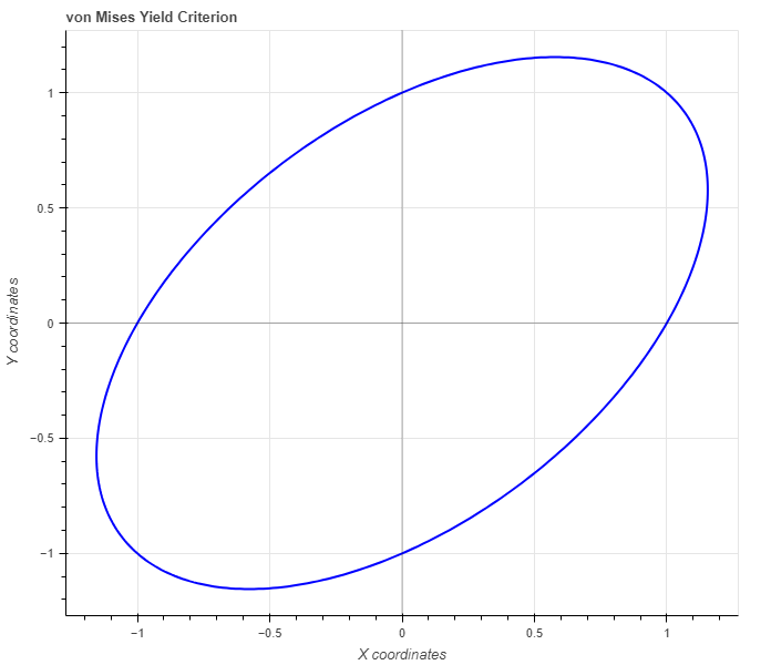
Figure 2: von Mises yield criterion representation. Ellipse curve intersects coordinates: (0,1) (1,1) (1,0) (0,-1) (-1,-1) (-1,0)
After you access uniform ellipse page you will find a button This button generates the ellipse as shown in Figure 2. When ellipse is added on the plot you can modify it by changing the color of the curve, line width and etc. You can also fill ellipse area with a color and modify it as you like.
You can also show or hide Tresca criterion, maximum shear stress in isotropic material, and modify this polyline as well as ellipse curve.
After you generate the ellipse you can add a pipe data by pressing a button and add a load case data by pressing . You can add up to 5 different pipe specifications and up to 20 different load cases.
In the pipe section you have 3 required parameters: Outside Diameter (OD), Inside Diameter (ID) and Yield Strength of the pipe material (YS).
There are 2 more optional parameters you may input as well: minimum Wall Thickness (mWT) and Corrosion Allowance (CA). Units for mWT is % and it is based on the specified manufacturing tolerance. Common number which is used for tubing and casing in the oil industry is 87,5%. Units for CA are either in or mm, depending which system you choose by pressing buttons Corrosion allowance is a measurement to the thickness of the wall. It is a metal loss throughout the lifespan of certain material in a certain conditions.
When you fill in all parameters for the pipe, press button. It is also a good practice to give a specific name for the pipe, for example: Tubing 4,5"-12,6#. This name will be shown on the generated report.
Now you can specify the loading parameters for the pipe if you press button. Here you have an option to enter internal pressure (IP), external pressure (EP) and axial load (Force) positive or negative value. Positive value of the Force parameter represents the tensile load and negative value represents the compressive load. If one the parameters should not be specified then type 0.
After you fill in all magnitudes of the load case, press button. You will not see any changes on the plot until you select the pipe under button for a specific pipe name from the list.
You can customize the load case by changing the specific parameters under button. There are 2 parameters that might catch your attention, show SF and connected. with. If you select show SF (Safety Factor) the line is drawn connecting the vertex of your load case and the curve of the ellipse. The safety factor value of the specific load case is then displayed in the legend of the plot. You can also modify that line as you wish. Connected with parameter available when you have 2 or more load cases and is useful to visualize the sequence of loading and check if any of the cases intersect the ellipse curve.
After you enter the required data for your analysis you can generate the report by pressing button. There you can fill the Project Name, Document Number, Created by and your Company Logo. You can also leave those fields blank and our company logo will be set on the report. To download the report you need to press button again. At the bottom of the export pop-up window you will find two html links. The first link is to download the report in PDF format and the other link is to download HTML plot, that might be useful to observe if you have high density data.
Below you may watch a short video tutorial of how to use the forms of this particular calculation.
Video: 1 Uniform Ellipse manual
von Mises yield criterion for tube loaded by internal and external pressure and axial stress, ISO 13679 or API RP 5C5 representation. This type of von Mises failure envelope is based on the method described in API 5C3 A.1.3.2.3.
The ellipse curve is actually represents the limit for a particular pipe size and consists of two curves, upper and lower curve. The Upper envelope curve is drawn on the top two quadrants, limiting the pipe in internal pressure and axial force, tension or compression. The lower envelope curve is drawn on the bottom two quadrants, limiting the pipe in external pressure and axial force, tension or compression. The points where both upper and lower curves bisect the X axis in the negative and positive regions (tensile force/compressive force) distort the form of the ellipse. Thicker pipe more visible distortion you may observe on the plot. See example below in the Figure 3.
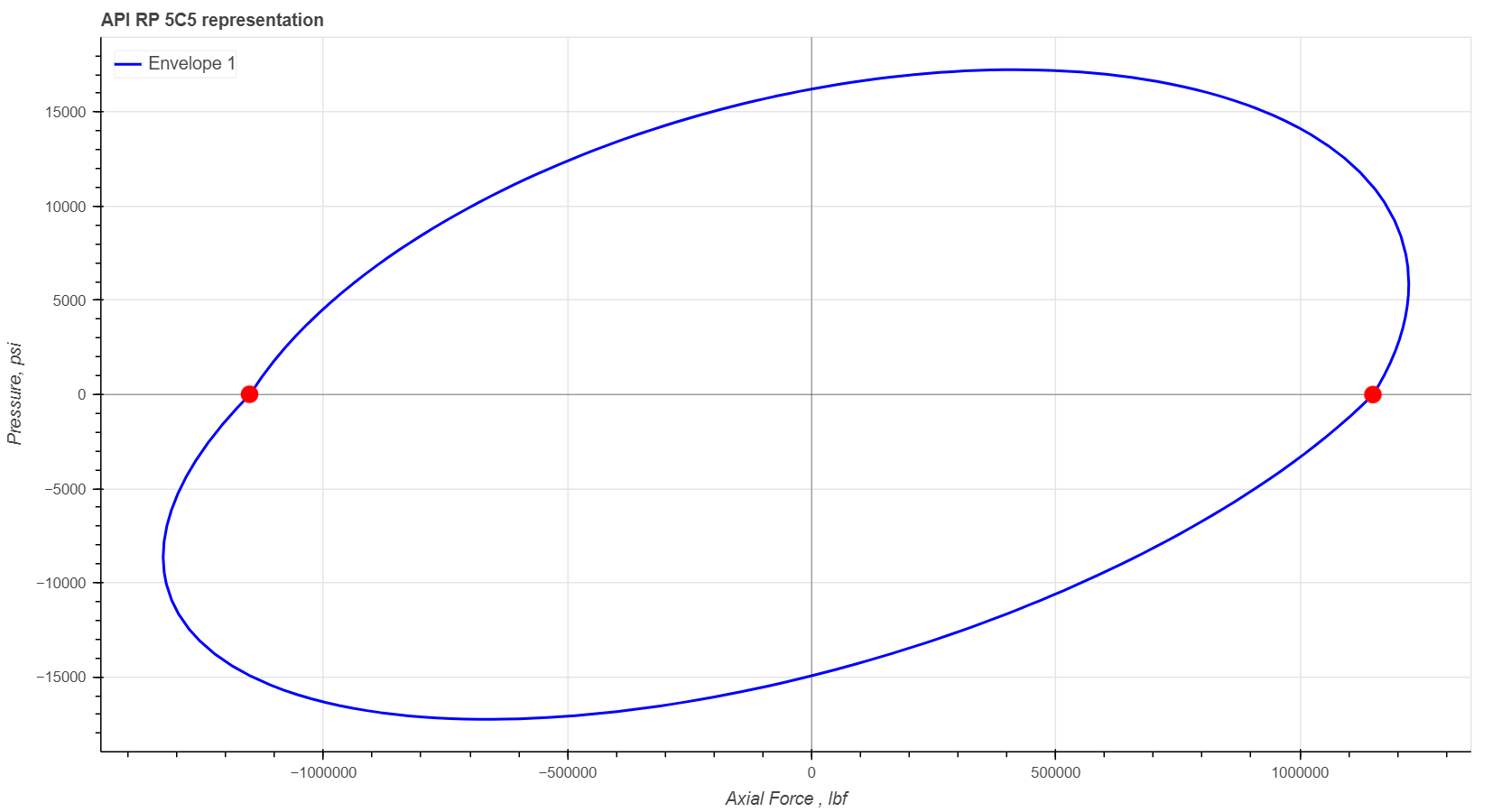
Figure 3: Performance envelope for the tube 7"-49.5#. Red marked vertices show where the curve is distorted due to a thick tubing wall. This is the reason we call it nonuniform ellipse.
After you access nonuniform ellipse page you will find two buttons and You can add up to 5 different pipe specifications and up to 20 different load cases. By adding multiple pipes to the plot you can easily compare them to each other to observe the boundaries and safe regions withing the same loading conditions. See example in the Figure 4.
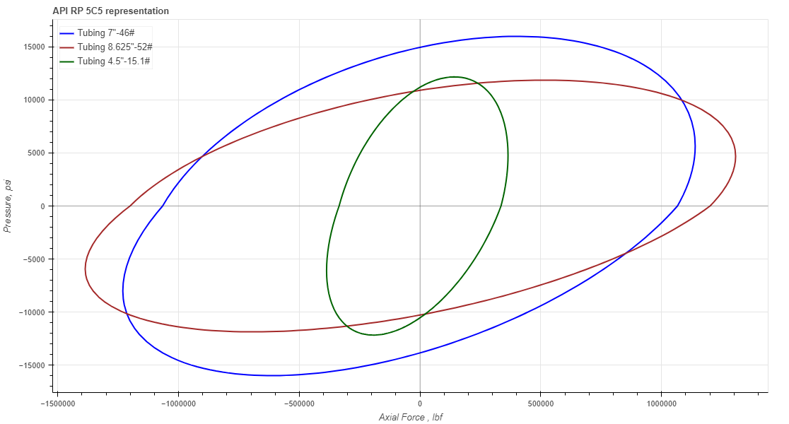
Figure 4: Performance envelopes for three different pipes on one plot: Tubing 7"-46# (blue), Tubing 8.625"-52# (brown) and Tubing 4.5"-15.1# (green).
In the pipe section you have 3 required parameters: Outside Diameter (OD), Inside Diameter (ID) and Yield Strength of the pipe material (YS).
There are 3 more optional parameters you may input as well: minimum Wall Thickness (mWT), Corrosion Allowance (CA) and Safety FActor (SF). Units for mWT is % and it is based on the specified manufacturing tolerance. Common number which is used for tubing and casing in the oil industry is 87,5%. Units for CA are either in or mm, depending which system you choose by pressing buttons Corrosion allowance is a measurement to the thickness of the wall. It is a metal loss throughout the lifespan of certain material in a certain conditions. The SF field gives you an option to reduce proportionally the envelope by the given factor.
Under button in the pipe section you show/hide multiple features for a particular envelope such as main vertices, proportional force limits (6 available), capped-ends limits and etc. All vertices and lines you can also customize with different color, type and size.
By opting to showcase the main vertices, you will witness 9 vertices positioned along the curve, revealing the precise boundaries of the specific pipe. See red dots not interesting with vertical line (force limits) on the Figure 5. By opting to showcase the force limits, you will witness 6 vertical lines expressed as percentages from the maximum tension and compression values for a specific pipe. Below under button you can change those percentages for specific values you need. See green dashed lines on the Figure 5. By opting to showcase the capped-ends, you will witness 2 vertical lines at the maximum internal and external peaks. See black dot-dash lines on the Figure 5.
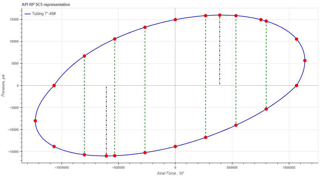
Figure 5: Performance envelopes for Tubing 7"-46# (blue), showing available features in the pipe section.
Now you can specify the loading parameters for the pipe if you press button. Here you have an option to enter a pressure magnitude (positive or negative) and axial load (Force) positive or negative value. Positive values for pressure field represent internal pressure and negative values represent external pressure. Positive value of the Force parameter represents the tensile load and negative value represents the compressive load. If one the parameters should not be specified then type 0.
You can customize the load case by changing the specific parameters under button. There are 2 parameters that might catch your attention, connected with and SF show with. If you select a pipe name under SF show with the line is drawn connecting the vertex of your load case and the curve of the selected ellipse. The safety factor value of the specific load case is then displayed in the legend of the plot. You can also modify that line as you wish. Connected with parameter available when you have 2 or more load cases and is useful to visualize the sequence of loading and check if any of the cases intersect the ellipse curve.
After you enter the required data for your analysis you can generate the report by pressing button. There you can fill the Project Name, Document Number, Created by and your Company Logo. You can also leave those fields blank and our company logo will be set on the report. To download the report you need to press button again. At the bottom of the export pop-up window you will find two html links. The first link is to download the report in PDF format and the other link is to download HTML plot, that might be useful to observe if you have high density data.
Below you may watch a short video tutorial of how to use the forms of this particular calculation.
Video: 2 Nonuniform Ellipse manual
von Mises yield criterion expressed in terms of internal and external pressure and effective stress (API 5C3 A.1.3.2.4).
A uniform circle has been pre-drawn on the Cartesian system, positioned at the coordinate system's origin, and with a radius of 1, as depicted in Figure 6. Due to the unequal ratio of our screens (not in a 1:1 aspect ratio), the circle will appear stretched along the X-axis. However, it is important to note that this visual effect does not impact the results.
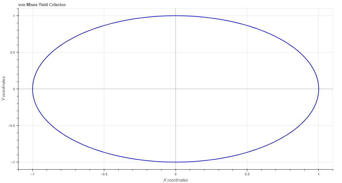
Figure 6: von Mises yield criterion representation (wide ratio) Circle curve intersects coordinates: (0,1) (1,0) (0,-1) (-1,0). Radius = 1
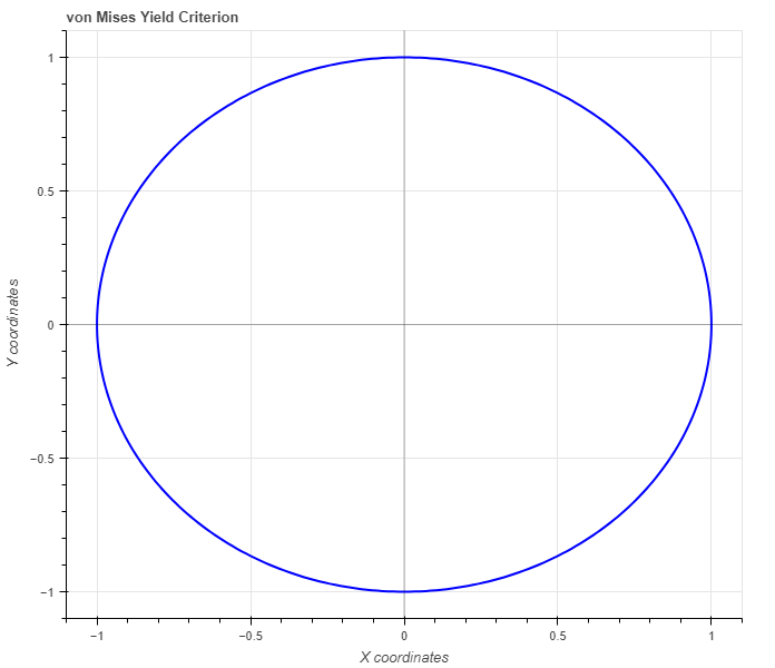
Figure 7: von Mises yield criterion representation (ratio 1:1) Circle shape is displayed when the internet browser has an equal ratio.
After you access uniform circle page you will find a button This button generates the ellipse as shown in Figure 6. When circle is added on the plot you can modify it by changing the color of the curve, line width and etc. You can also fill circle area with a color and modify it as you like.
After you generate the circle you can add a pipe data by pressing a button and add a load case data by pressing . You can add up to 5 different pipe specifications and up to 20 different load cases.
In the pipe section you have 3 required parameters: Outside Diameter (OD), Inside Diameter (ID) and Yield Strength of the pipe material (YS).
There are 2 more optional parameters you may input as well: minimum Wall Thickness (mWT) and Corrosion Allowance (CA). Units for mWT is % and it is based on the specified manufacturing tolerance. Common number which is used for tubing and casing in the oil industry is 87,5%. Units for CA are either in or mm, depending which system you choose by pressing buttons Corrosion allowance is a measurement to the thickness of the wall. It is a metal loss throughout the lifespan of certain material in a certain conditions.
When you fill in all parameters for the pipe, press button. It is also a good practice to give a specific name for the pipe, for example: Tubing 4,5"-12,6#. This name will be shown on the generated report.
Now you can specify the loading parameters for the pipe if you press button. Here you have an option to enter internal pressure (IP), external pressure (EP) and axial load (Force) positive or negative value. Positive value of the Force parameter represents the tensile load and negative value represents the compressive load. If one the parameters should not be specified then type 0.
After you fill in all magnitudes of the load case, press button. You will not see any changes on the plot until you select the pipe under button for a specific pipe name from the list.
You can customize the load case by changing the specific parameters under button. There are 2 parameters that might catch your attention, show SF and connected. with. If you select show SF (Safety Factor) the line is drawn connecting the vertex of your load case and the curve of the circle. The safety factor value of the specific load case is then displayed in the legend of the plot. You can also modify that line as you wish. Connected with parameter available when you have 2 or more load cases and is useful to visualize the sequence of loading and check if any of the cases intersect the circle curve.
After you enter the required data for your analysis you can generate the report by pressing button. There you can fill the Project Name, Document Number, Created by and your Company Logo. You can also leave those fields blank and our company logo will be set on the report. To download the report you need to press button again. At the bottom of the export pop-up window you will find two html links. The first link is to download the report in PDF format and the other link is to download HTML plot, that might be useful to observe if you have high density data.
Below you may watch a short video tutorial of how to use the forms of this particular calculation.
Video: 3 Uniform Circle manual