
Tip
See our video guides for quick tutorials that walk you through Sigmacalx basic functionalities and concepts. This is the easiest and quickest way to get going with Sigmacalx forms.
Three key mechanical stresses that can be imposed on an object with a cylindrical shape are as follows:
Formulas to calculate those stresses are taken from API 5C3 standard (A.1.2.2), and are valid for "thick-walled" pressure vessels with their wall thickness greater than one-tenth of the overall diameter.
Hoop stress, also referred to as circumferential stress, is a type of normal stress that occurs in a cylindrical or circular structure, such as a pipe or a hoop. It is the stress that acts in the tangential direction around the circumference of the object.
Hoop stress arises as a result of internal or external pressure applied to the cylindrical object. When a cylindrical structure is subjected to an internal pressure, such as fluid or gas pressure, the material experiences a tendency to expand outward. This expansion creates a force that acts circumferentially around the cylinder, causing the material to be stressed in the tangential direction.
The magnitude of the hoop stress is directly related to the internal or external pressure applied to the cylinder and the radius of the object. The hoop stress is highest at the innermost surface of the cylinder and gradually decreases towards the outer surface.
Hoop stress is a critical factor in the design and analysis of cylindrical structures, as it helps determine the structural integrity and the ability of the object to withstand the pressure load without failure.
Upon accessing the Circumferential (or hoop) Stress page, you will encounter two buttons: and These buttons allow you to include up to 5 distinct pipe specifications and up to 20 different load cases. By incorporating multiple pipes and load cases into the plot, you can conveniently compare them to one another, enabling the observation of boundaries and safe regions. An example illustrating this can be seen in Figure 8.
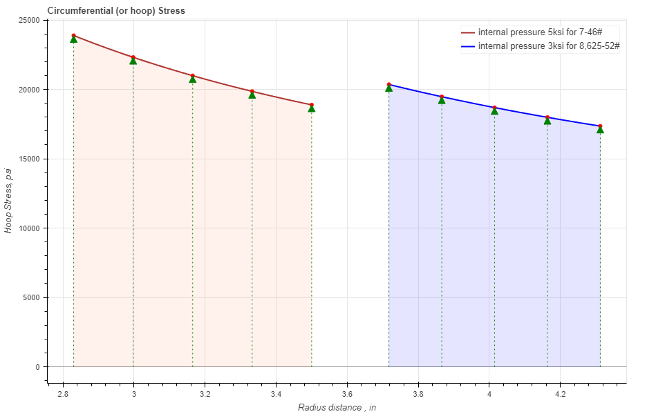
Figure 8: Two hoop stress curves are presented, representing the stress distribution across the wall of two tubing sizes exposed to varying internal pressure levels.
For enhanced comprehension of the stress distribution throughout the thickness, you have the option to simultaneously exhibit the radial cross-section of the pipe alongside a hoop stress curve.
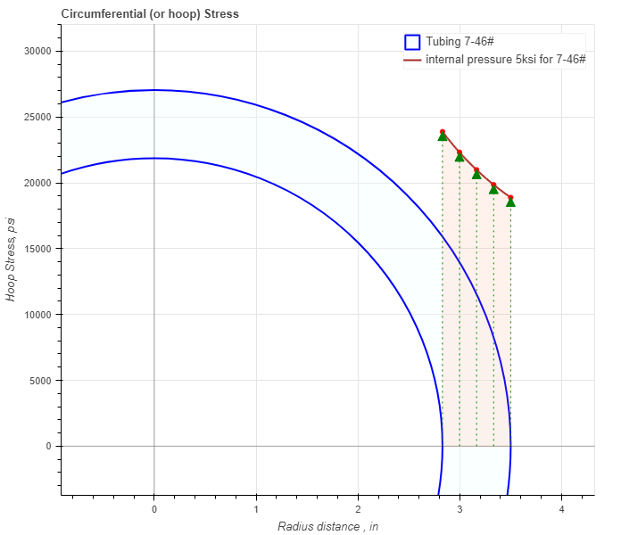
Figure 9: Hoop stress curve with a specified pipe, representing the stress distribution across the wall of a particular tubing size exposed to internal pressure.
In the pipe section you have 2 required parameters: Outside Diameter (OD) and Inside Diameter (ID)
There are 2 more optional parameters you may input on the tubing section: minimum Wall Thickness (mWT) and Corrosion Allowance (CA). Units for mWT is % and it is based on the specified manufacturing tolerance. Common number which is used for tubing and casing in the oil industry is 87,5%. Units for CA are either in or mm, depending which system you choose by pressing buttons Corrosion allowance is a measurement to the thickness of the wall. It is a metal loss throughout the lifespan of certain material in a certain conditions.
When pipe cross-section is added on the plot you can modify it by changing the color of the curve, line width and etc. You can also fill the cross-section area with a color and modify it as you like.
When you fill in all parameters for the pipe, press button. It is also a good practice to give a specific name for the pipe, for example: Tubing 7"-46#. This name will be shown on the generated report and on the selection menu in the load section.
Now you can specify the loading parameters for the pipe if you press button. Here you have an option to enter internal pressure (IP), external pressure (EP) and select the pipe you want to apply the loads for. If IP or EP should not be specified then type 0.
After you fill in all magnitudes of the load case, press button. You will not see any changes on the plot until you select the specific pipe name from the list.
You can customize the load case by changing the specific parameters under button. There is one parameter that might catch your attention, POI (Point of Interest). This parameter provides you with a distinct stress value corresponding to a distance between the internal and external radii that you input into the designated field.
After you enter the required data for your analysis you can generate the report by pressing button. There you can fill the Project Name, Document Number, Created by and your Company Logo. You can also leave those fields blank and our company logo will be set on the report. To download the report you need to press button again. At the bottom of the export pop-up window you will find two html links. The first link is to download the report in PDF format and the other link is to download HTML plot, that might be useful to observe if you have high density data.
Below you may watch a short video tutorial of how to use the forms of this particular calculation.
Video: 4 Circumferential (or hoop) Stress manual
Radial stress within a pipe is the effective stress that operates in the direction perpendicular to the longitudinal axis of the pipe, commonly referred to as the radial direction. This stress is termed "radial stress" due to its orientation along this radial direction.
Upon accessing the Radial Stress page, you will encounter two buttons: and These buttons allow you to include up to 5 distinct pipe specifications and up to 20 different load cases. By incorporating multiple pipes and load cases into the plot, you can conveniently compare them to one another, enabling the observation of boundaries and safe regions. An example illustrating this can be seen in Figure 10.
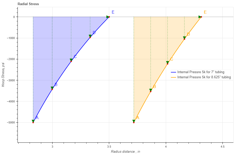
Figure 10: Two radial stress curves are presented, representing the stress distribution across the wall of two tubing sizes exposed to varying internal pressure levels.
For enhanced comprehension of the stress distribution throughout the thickness, you have the option to simultaneously exhibit the radial cross-section of the pipe alongside a radial stress curve.
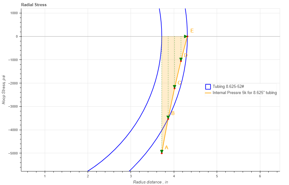
Figure 11: Radial stress curve with a specified pipe, representing the stress distribution across the wall of a particular tubing size exposed to internal pressure.
In the pipe section you have 2 required parameters: Outside Diameter (OD) and Inside Diameter (ID)
There are 2 more optional parameters you may input on the tubing section: minimum Wall Thickness (mWT) and Corrosion Allowance (CA). Units for mWT is % and it is based on the specified manufacturing tolerance. Common number which is used for tubing and casing in the oil industry is 87,5%. Units for CA are either in or mm, depending which system you choose by pressing buttons Corrosion allowance is a measurement to the thickness of the wall. It is a metal loss throughout the lifespan of certain material in a certain conditions.
When pipe cross-section is added on the plot you can modify it by changing the color of the curve, line width and etc. You can also fill the cross-section area with a color and modify it as you like.
When you fill in all parameters for the pipe, press button. It is also a good practice to give a specific name for the pipe, for example: Tubing 7"-46#. This name will be shown on the generated report and on the selection menu in the load section.
Now you can specify the loading parameters for the pipe if you press button. Here you have an option to enter internal pressure (IP), external pressure (EP) and select the pipe you want to apply the loads for. If IP or EP should not be specified then type 0.
After you fill in all magnitudes of the load case, press button. You will not see any changes on the plot until you select the specific pipe name from the list.
You can customize the load case by changing the specific parameters under button. There is one parameter that might catch your attention, POI (Point of Interest). This parameter provides you with a distinct stress value corresponding to a distance between the internal and external radii that you input into the designated field.
After you enter the required data for your analysis you can generate the report by pressing button. There you can fill the Project Name, Document Number, Created by and your Company Logo. You can also leave those fields blank and our company logo will be set on the report. To download the report you need to press button again. At the bottom of the export pop-up window you will find two html links. The first link is to download the report in PDF format and the other link is to download HTML plot, that might be useful to observe if you have high density data.
Below you may watch a short video tutorial of how to use the forms of this particular calculation.
Video: 5 Radial Stress manual
Longitudinal stress pertains to the stress or force encountered by a material along its longitudinal axis, the axis that runs parallel to the length of the object.
In the realm of engineering and materials science, longitudinal stress frequently corresponds to the tensile or compressive forces exerted along an object's length. Tensile stress emerges when a material is stretched or pulled apart along its length, whereas compressive stress arises when the material is compressed or pressed together along its length.
Upon accessing the Longitudinal Stress page, you will encounter two buttons: and These buttons allow you to include up to 5 distinct pipe specifications and up to 20 different load cases. By incorporating multiple pipes and load cases into the plot, you can conveniently compare them to one another, enabling the observation of boundaries and safe regions. An example illustrating this can be seen in Figure 12.
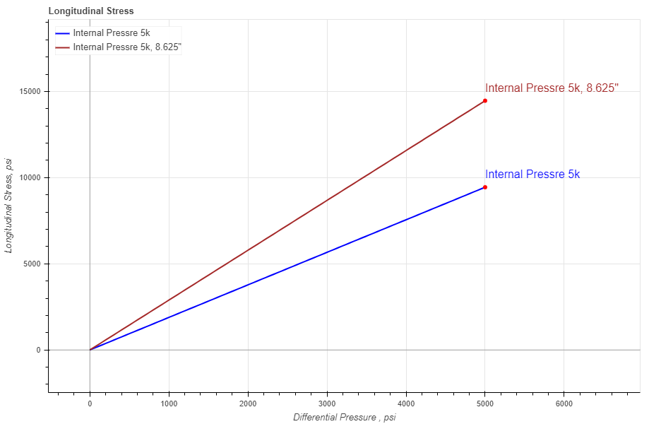
Figure 12: Two longitudinal stresses are presented, representing the stress distribution depending on the differential pressure of two tubing sizes exposed to varying internal pressure levels.
In the pipe section you have 2 required parameters: Outside Diameter (OD) and Inside Diameter (ID)
There are 2 more optional parameters you may input on the tubing section: minimum Wall Thickness (mWT) and Corrosion Allowance (CA). Units for mWT is % and it is based on the specified manufacturing tolerance. Common number which is used for tubing and casing in the oil industry is 87,5%. Units for CA are either in or mm, depending which system you choose by pressing buttons Corrosion allowance is a measurement to the thickness of the wall. It is a metal loss throughout the lifespan of certain material in a certain conditions.
When you fill in all parameters for the pipe, press button. It is also a good practice to give a specific name for the pipe, for example: Tubing 7"-46#. This name will be shown on the generated report and on the selection menu in the load section.
Now you can specify the loading parameters for the pipe if you press button. Here you have an option to enter internal pressure (IP), external pressure (EP) and select the pipe you want to apply the loads for. If IP or EP should not be specified then type 0.
After you fill in all magnitudes of the load case, press button. You will not see any changes on the plot until you select the specific pipe name from the list.
You can customize the load case by changing the specific parameters under button. Here you can choose a color, type and width for the stress line.
After you enter the required data for your analysis you can generate the report by pressing button. There you can fill the Project Name, Document Number, Created by and your Company Logo. You can also leave those fields blank and our company logo will be set on the report. To download the report you need to press button again. At the bottom of the export pop-up window you will find two html links. The first link is to download the report in PDF format and the other link is to download HTML plot, that might be useful to observe if you have high density data.
Below you may watch a short video tutorial of how to use the forms of this particular calculation.
Video: 6 Longitudinal Stress manual